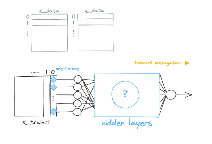
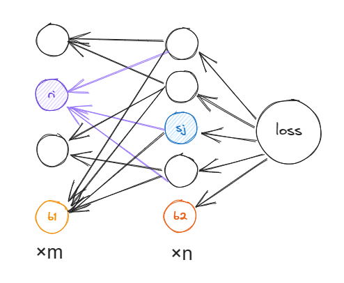
definitialize_network(layer_dims): layers = [] input_layer = [] # input layer: with no weight for num inrange(layer_dims[0]): input_layer.append(Neuron(weight_size=0)) layers.append(input_layer)
# other layers: with weight size equal to the neurons in the layer before for i inrange(1, len(layer_dims)): layer = [] for num inrange(layer_dims[i]): layer.append( Neuron(weight_size=layer_dims[i-1], input=layers[i-1])) layers.append(layer)
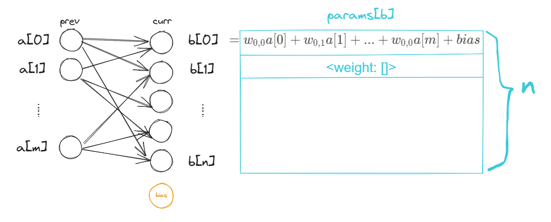
# hidden layers for layer_idx inreversed(range(0, len(layers)-2)): for neuron_idx inrange(len(layers[layer_idx])): layers[layer_idx][neuron_idx].delta =\ np.sum([n.delta*n.weight[neuron_idx]*tanh_derivative(n.output) for n in layers[layer_idx+1]]) for neuron_idx inrange(len(layers[layer_idx+1])): neuron = layers[layer_idx+1][neuron_idx] neuron.weight -= np.multiply([n.output for n in layers[layer_idx]], neuron.delta * tanh_derivative(neuron.output)*learning_rate) biases[layer_idx] -= neuron.delta * \ tanh_derivative(neuron.output)*learning_rate
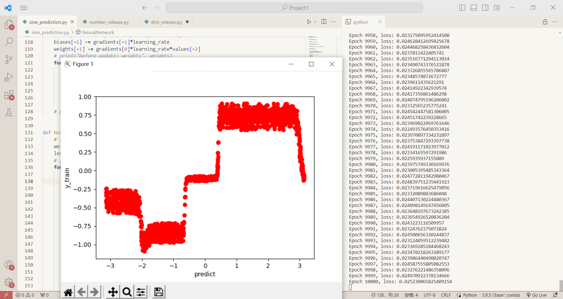
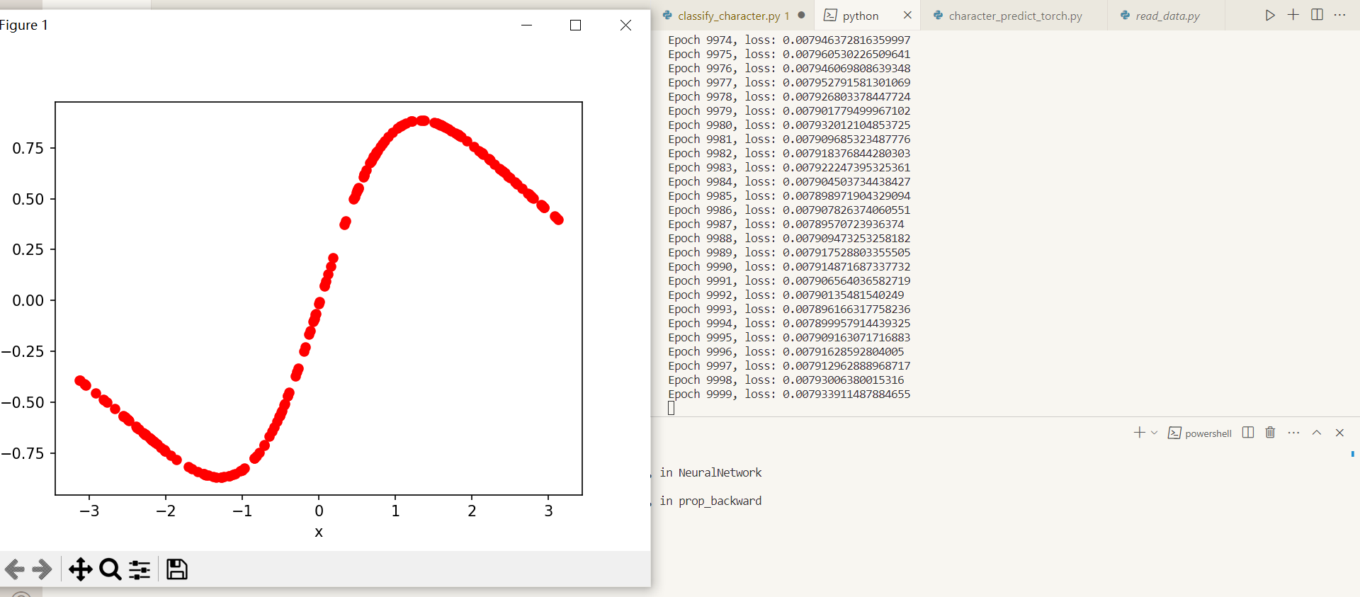
defNeuralNetwork(X_train, y_train, layer_dims, epochs=10000, batch_size=20): # 1. initialize the network layers, biases = initialize_network(layer_dims) # 2. train loss = 1 for epoch inrange(epochs): learning_rate = 0.0005 if loss < 0.05: learning_rate = 0.00005 elif loss < 0.030: learning_rate = 0.00001 elif loss < 0.015: learning_rate = 0.000002 elif loss < 0.008: learning_rate = 0.0000005 # concatenate and shuffle the data train_data = np.column_stack((X_train, y_train)) np.random.shuffle(train_data) # retrieve x and y from concatenated data x = train_data.T[0] y = train_data.T[1] losses = [] predictions = [] for i inrange(x.__len__()): # prop forward prediction = prop_forward([x[i]], layers, biases) predictions.append(prediction) losses.append(mse_loss(prediction, y[i])) if i % batch_size == 0: prop_backward(y[i], layers, biases, learning_rate) # compute loss loss = np.mean(losses) if (epoch+1) % 1000 == 0: plt.clf() plt.plot(x, predictions, "ro") plt.xlabel("x") plt.ylabel("predict") plt.show() print(f"Epoch {epoch+1}, loss: {loss}")
if __name__ == "__main__": X_train, y_train = produce_data(200)
defload_images(data_dir): data = [] for i inrange(1, 13): folder_path = os.path.join(data_dir, str(i)) for pic in os.listdir(folder_path): data.append([os.path.join(folder_path, pic), i]) return data
defrelu(x): return np.maximum(0, x)
defrelu_derivative(x): if x > 0: return1 else: return0
definitialize_network(layer_dims): layers = [] input_layer = [] # input layer: with no weight for num inrange(layer_dims[0]): input_layer.append(Neuron(weight_size=0)) layers.append(input_layer)
# other layers: with weight size equal to the neurons in the layer before for i inrange(1, len(layer_dims)): layer = [] for num inrange(layer_dims[i]): layer.append( Neuron(weight_size=layer_dims[i-1], input=layers[i-1])) layers.append(layer)
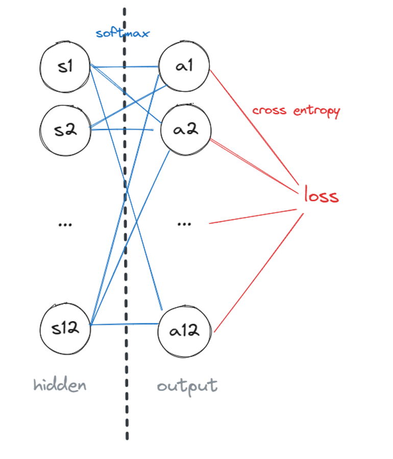
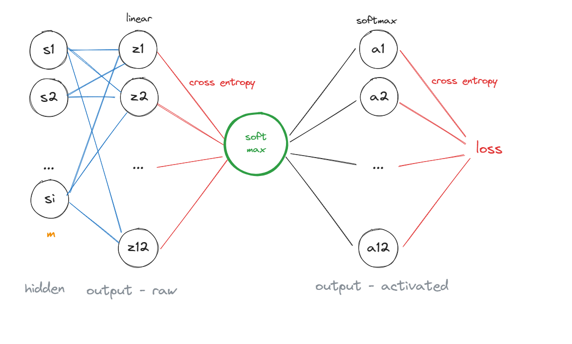
defprop_backward(target, layers, biases, learning_rate=0.01): # output layer for neuron_idx inrange(len(layers[-1])): layers[-1][neuron_idx].delta = (layers[-1] [neuron_idx].output-target)[neuron_idx] for neuron_idx inrange(len(layers[-2])): layers[-2][neuron_idx].delta = np.sum( [n.delta*n.weight[neuron_idx]for n in layers[-1]]) for neuron_idx inrange(len(layers[-1])): neuron = layers[-1][neuron_idx] neuron.weight -= np.multiply([n.output for n in layers[-2]], neuron.delta * learning_rate)
# hidden layers for layer_idx inreversed(range(0, len(layers)-2)): for neuron_idx inrange(len(layers[layer_idx])): layers[layer_idx][neuron_idx].delta =\ np.sum([n.delta*n.weight[neuron_idx]*relu_derivative(n.output) for n in layers[layer_idx+1]]) for neuron_idx inrange(len(layers[layer_idx+1])): neuron = layers[layer_idx+1][neuron_idx] neuron.weight -= np.multiply([n.output for n in layers[layer_idx]], neuron.delta * relu_derivative(neuron.output)*learning_rate) biases[layer_idx] -= neuron.delta * \ relu_derivative(neuron.output)*learning_rate biases[0] = 0
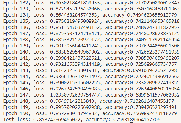
# 2. train loss = 100 for epoch inrange(epochs): learning_rate = 0.00005 if loss < 1: learning_rate = 0.00001 elif loss < 0.8: learning_rate = 0.000002 # concatenate and shuffle the data train_data = np.column_stack((X_train, y_train)) np.random.shuffle(train_data) # retrieve x and y from concatenated data x = train_data.T[0] y = train_data.T[1] losses = [] predictions = [] hit = 0 for i inrange(x.__len__()): prediction = prop_forward(x[i], layers, biases) predictions.append(prediction) if np.argmax(y[i]) == np.argmax(prediction): hit += 1 losses.append(ce_loss(prediction, y[i])) if i % batch_size == 0: prop_backward(y[i], layers, biases, learning_rate)
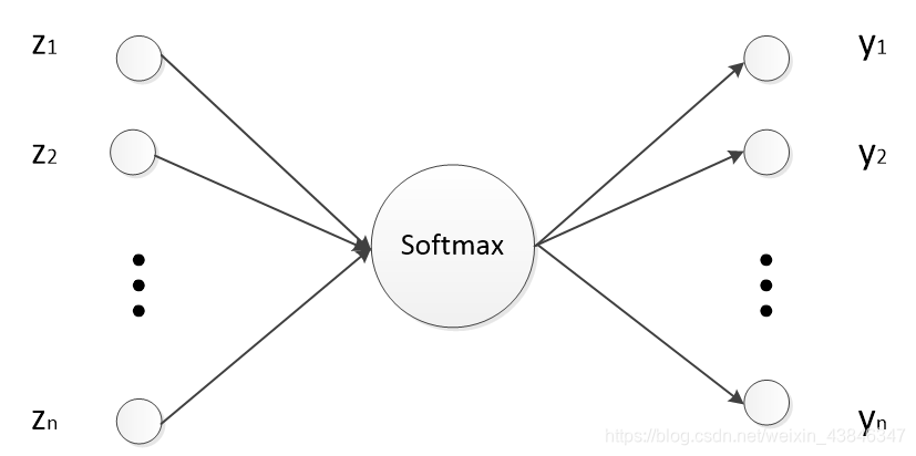
# compute loss loss = np.mean(losses) print(f"Epoch {epoch+1}, loss: {loss}, accuracy:{hit/len(y)}") # 3. test test_data = np.column_stack((X_test, y_test)) test_x = test_data.T[0] test_y = test_data.T[1] test_losses = [] test_predictions = [] test_hit = 0 for i inrange(test_x.__len__()): prediction = prop_forward(test_x[i], layers, biases) test_predictions.append(prediction) if np.argmax(test_y[i]) == np.argmax(prediction): test_hit += 1 test_losses.append(ce_loss(prediction, test_y[i])) if i % batch_size == 0: prop_backward(test_y[i], layers, biases, learning_rate)
# compute loss test_loss = np.mean(test_losses) print(f"Test loss: {test_loss}, accuracy:{test_hit/len(test_y)}")
defimage_to_array(data_dir): img_list = load_images(data_dir) data = [] onehot_mat = np.eye(12) for i inrange(len(img_list)): img_name = img_list[i][0] img_arr = imageio.v2.imread(img_name) img_data = 255.0-img_arr.reshape(784) label = img_list[i][1]-1 data.append([img_data, onehot_mat[label]]) data = np.array(data, dtype=object) np.random.shuffle(data) x = data.T[0] y = data.T[1] return x, y